Tensor trains and quantum-inspired compression
Ranks, cores, deployment trade-offs
The Problem
Where compression pays
Large language models dominate memory bandwidth in inference clusters. Even modest fractional savings per layer propagate to measurable power and leasing savings when multiplied by millions of queries.
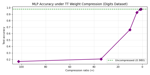
The compression chapter explains tensor trains as a rank-controlled approximation of weight tensors, then measures accuracy versus compression on a toy classifier so the mechanics are visible without multi-node clusters.
The Challenge
Rank is a budget knob, not a hyperparameter you ignore
The Challenge
Accuracy versus footprint
Lower rank reduces parameters but can erase useful curvature in the decision surface. Plot both compression ratio and validation accuracy as functions of rank—exactly the Pareto reasoning operations teams need.
Questions operations should ask
- Which layers are safe to compress first given attention patterns?
- What offline acceptance suite gates a compressed checkpoint?
- What rollback artefact ships alongside the compressed weights?
The Solution
TT decomposition + reconstruction error budget
The Solution
Why “quantum-inspired” belongs in this saga
The tensor network literature matured in many-body physics. Machine learning reuses the factorisation as an engineering tool. You can deliver value without claiming a quantum speedup.
Implementation
Reshape, decompose, rebuild, measure
Implementation
The companion repository uses TensorLy-style calls; the sketch below keeps names library-agnostic so you can map to your stack.
Calibrate r against a validation metric, not matrix Frobenius error alone.
W_tensor = weight_matrix.reshape(factor_dims)  # e.g. (4,16,4,16)
cores = tensor_train_decompose(W_tensor, rank=[1, r, r, r, 1])
W_hat = tensor_train_reconstruct(cores).reshape_as(weight_matrix)
ratio = weight_matrix.numel() / sum(c.numel() for c in cores)
Pair with latency measurements if you approach production.
logits_full = model(x)
logits_tt = model_with_tt_layer(x)
acc_drop = accuracy(logits_full, y) - accuracy(logits_tt, y)Summary
Toy benchmark: 0.9796 full vs 0.9278 TT rank-8, ~4.5× compression
Summary
How to cite these figures
They originate from a small classifier sanity check in the workshop materials, not from a frontier LLM. Use them to explain the shape of the trade-off curve, then rerun the pipeline on your own weights.
Continue this saga
Next chapter: Deployment and governance.