The Challenge

What goes wrong in practice

If penalties are too weak, the best energy can correspond to an illegal portfolio. If penalties are too strong, the landscape flattens everywhere feasible and samplers stall. The toy examples use modest numbers so those behaviours are visible on a laptop.

The Solution

From QUBO to Hamiltonian language

After constructing Q, you map to Ising couplings for use in QAOA-style circuits. The pedagogical point is structural: the same Q appears in classical energy minimisation and in quantum expectation training—only the state preparation changes.

What the QUBO is actually counting

Write binary decision variables \(x_i \in \{0,1\}\) for “include asset \(i\)”. Expected portfolio return is \(\mu^\top x\) up to sign conventions in your encoding. Sample covariance \(\Sigma\) contributes \(\sum_{i,j}\Sigma_{ij} x_i x_j\), which is the standard Markowitz risk quadratic once you fix whether you minimise risk or maximise a penalised objective. Cardinality and sector constraints become additional quadratic or linear penalty terms so that illegal patterns sit at high classical energy.

That object is deliberately pseudo-Boolean: it is the same mathematical species as MaxCut-style problems, so any library that accepts Q matrices or Ising \((h,J)\) pairs can evaluate your portfolio model without knowing it came from finance.

QAOA as a disciplined sampler, not a guarantee

Mapping \(x_i = (1 - z_i)/2\) for spins \(z_i \in \{-1,+1\}\) yields local fields and pairwise couplings. A depth-\(p\) QAOA applies alternating layers: a phase operator \(\exp(-\mathrm{i} \gamma_k H_C)\) derived from the cost Hamiltonian, and a mixer \(\exp(-\mathrm{i} \beta_k H_B)\) that spreads amplitude across computational basis states. The variational state is therefore a structured superposition; measuring it produces bitstrings that you decode back to portfolios.

The mixer’s job is to move probability mass between candidates after the cost layer has imprinted phases that separate low-energy from high-energy strings. Neither layer, by itself, solves the combinatorial problem: the classical optimiser still searches \((\gamma,\beta)\) using shot noise or exact simulation, and you still verify each draw against business rules.

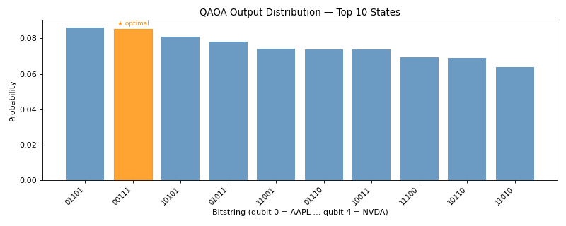
Interpreting sampler output

Good variational parameters may still leave modest mass on the global optimum; that is why the narrative overlays classical enumeration for small n. When n grows, replace enumeration with a trusted solver but keep the Q matrix identical.

Implementation

The sketch condenses Part B: assemble Q from returns and covariance, translate to Ising (h, J), wrap a shallow QAOA ansatz, and optimise γ/β or equivalent parameters with a classical loop.

Keep offset explicit when comparing energies to a classical QUBO solver.

def portfolio_qubo(mu, Sigma, budget, risk_w, pen):
    # diagonal encourages high expected return, off-diagonals penalise covariance,
    # penalty terms enforce cardinality — see companion code for full expansion
    Q = assemble_Q(mu, Sigma, budget, risk_w, pen)
    h, J, offset = qubo_to_ising(Q)
    return Q, h, J, offset

def qaoa_energy(gamma, beta, h, J, shots):
    return hardware_or_sim_expectation(gamma, beta, h, J, shots=shots)

Always plot histogram mass near best_cost; do not report only the best draw.

best_cost, best_bits = brute_force_minimize(Q)
hist = variational_sample(gamma, beta, n_shots=4096)
compare_histogram_to_best(hist, best_cost)

Portfolio selection (companion code)

Summary

How to narrate the gap

Those numbers come from a deliberately small universe where classical enumeration is trustworthy. They illustrate that variational depth and parameter initialisation matter, not that “quantum loses.” Present them as a stress test of your encoding and baseline pipeline.

Next chapter

The following story swaps the business object but keeps the mathematics: logistics routes instead of securities, still ending in bitstrings, penalties, and readout checks.