Hybrid classifier stack

Quantum layer and classical head

The Problem

What “hybrid” means operationally

Batch tensors enter a classical feature pipeline, pass through a parametrized quantum map implemented as a differentiable circuit, then through a classical head (often linear) that produces logits or regression outputs. Gradients flow end-to-end; the optimiser updates both classical and quantum parameters unless you freeze subsets deliberately.

The toy dataset stays modest so you can focus on diagnostics: training versus validation curves, decision boundaries, and sensitivity to random seeds.

The Challenge

Shot noise meets minibatches

The Challenge

Interactions to watch

Finite shots inject gradient variance. Small batch sizes amplify that variance. The result can be surprisingly brittle learning even when the circuit diagram looks elegant.

Stabilisation checklist

Shot budget: tie shot counts to gradient variance targets, not round numbers.

Baseline parity: mirror preprocessing and augmentation exactly for the classical model.

Stopping: define when extra epochs cannot justify operator time.

The Solution

Evidence is the learning trace, not the final integer accuracy

The Solution

How Arraxis-style reviews read the result

Ask for the full curves first. A single held-out accuracy without variance bands is insufficient when shot noise is present. If the baseline wins within noise bands, the correct outcome is often “park the quantum branch” rather than tweak marketing language.

Loss and accuracy traces for hybrid training (illustrative run)

Implementation

End-to-end forward pass

Implementation

The following mirrors the classifier block: embedding, entangling layers, measurement, classical head, loss.

Batching requires stacking qnode calls or using TorchLayer; see companion code for the idiomatic pattern.

Hybrid module outline

import pennylane as qml
import torch
import torch.nn as nn

dev = qml.device("default.qubit", wires=4)

@qml.qnode(dev, interface="torch", diff_method="backprop")
def qnn(x, w):
    qml.AngleEmbedding(x, wires=range(4))
    qml.StronglyEntanglingLayers(w, wires=range(4))
    return [qml.expval(qml.PauliZ(i)) for i in range(4)]

class HybridClassifier(nn.Module):
    def __init__(self):
        super().__init__()
        self.w = nn.Parameter(0.01 * torch.randn(2, 4, 3))
        self.head = nn.Linear(4, 3)

    def forward(self, x):
        z = torch.stack(qnn(x, self.w))
        return self.head(z)

Hybrid classifier (companion code)

Summary

Illustrative metrics from a recorded run

Summary

Numbers to cite with care

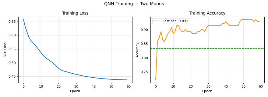
One stored evaluation on the toy split reported about 0.833 baseline test accuracy with late-training loss near 0.44 and training accuracy near 0.94. Use these as order-of-magnitude anchors only—your dataset will move them.

The actionable conclusion is methodological: insist on paired plots and seed sweeps before any procurement conversation.

Continue this saga

Next chapter: Finance: portfolio as a QUBO.